Water-bridge Interactions#
This tutorial showcases how to use ProLIF to generate an interaction fingerprint including water-mediated hydrogen-bond interactions, and analyze the interactions for a ligand-protein complex.
Preparation for MD trajectory#
Let’s start by importing MDAnalysis and ProLIF to read our tutorial files and create selections for the ligand, protein and water.
Important
It is advised to select for the protein and water selection only the residues in close distance to the ligand, else the generation of the fingerprint will be time consuming due to the amount of analyzed atoms.
For the selection of the protein in this tutorial we only select the residues around 12.0 Å of the ligand.
Tip
For the water component it is possible to update the AtomGroup distance-based selection at every frame,
which is convenient considering the large movements of water molecules during most simulations.
Do not use updating=True for the protein selection, it will produce wrong results.
For the water selection we select the water residues around 8 Å of the ligand or protein. You may adjust this distance threshold based on whether you’re investigating higher-order water-mediated interactions (which require a higher threshold to select all relevant waters) or not.
import MDAnalysis as mda
import pandas as pd
import prolif as plf

# load example topology and trajectory
u = mda.Universe(plf.datafiles.WATER_TOP, plf.datafiles.WATER_TRAJ)

# create selections for the ligand and protein
ligand_selection = u.select_atoms("resname QNB")
protein_selection = u.select_atoms(
    "protein and byres around 12 group ligand",
    ligand=ligand_selection,
)
water_selection = u.select_atoms(
    "resname TIP3 and byres around 8 (group ligand or group pocket)",
    ligand=ligand_selection,
    pocket=protein_selection,
    updating=True,
)
ligand_selection, protein_selection, water_selection
/home/docs/checkouts/readthedocs.org/user_builds/prolif/envs/302/lib/python3.11/site-packages/MDAnalysis/topology/TPRParser.py:161: DeprecationWarning: 'xdrlib' is deprecated and slated for removal in Python 3.13
  import xdrlib
(<AtomGroup with 49 atoms>,
 <AtomGroup with 1832 atoms>,
 <AtomGroup with 1011 atoms, with selection 'resname TIP3 and byres around 8 (group ligand or group pocket)' on the entire Universe.>)
Important
Note that the protein selection will only select residues around 12Å of the ligand on the first frame. If your ligand or protein moves significantly during the simulation and moves outside of this 12Å sphere, it may be more relevant to perform this selection multiple times during the simulation to encompass all the relevant residues across the entire trajectory.
To this effect, you can use select_over_trajectory():
protein_selection = plf.select_over_trajectory(
    u,
    u.trajectory[::10],
    "protein and byres around 12 group ligand",
    ligand=ligand_selection,
)
Preparation for docking poses#
To run a water-bridge analysis with ProLIF for a PDB file and docking poses, you will need
to create 3 objects: a protein molecule (plf.Molecule), a collection of ligand molecules
(e.g. a list of plf.Molecule), and a water molecule (plf.Molecule).
To create the protein and ligand(s) for your use case, refer to the docking tutorial.
Warning
To keep the size of test files to a minimum, here we will create molecules directly from the MD trajectory above, instead of using PDB/MOL2/SDF/PDBQT files. Please follow the instructions given in the relevant tutorial closely instead.
# create list of ligand poses for each frame in the MD trajectory
ligand_poses = [plf.Molecule.from_mda(ligand_selection) for ts in u.trajectory]
# create protein with waters
solvated_protein_mol = plf.Molecule.from_mda(protein_selection + water_selection)
We can now split our solvated protein into its separate components:
water_mol, protein_mol = plf.split_molecule(
    solvated_protein_mol, lambda resid: resid.name == "TIP3"
)
Analysis#
Now we perform the calculation of the interactions. In this tutorial we only focus on the water bridge interactions, but you can also include the other typical ligand-protein interactions in the list of interactions.
Important
When using WaterBridge, you must specify the water parameter with either your atomgroup selection
if using an MD trajectory, or the water molecule if using PDB/docking files.
By default, the WaterBridge interaction will only look at bridges including a single water molecule, i.e. ligand---water---protein.
Here, we will look at the water bridges up to order 3 (i.e. there can be up to 3 water molecules),
for this we explicitely provide order=3 in the parameters of the WaterBridge interaction (defaults to 1).
# for docking poses, replace water_selection with water_mol
fp = plf.Fingerprint(
    ["WaterBridge"], parameters={"WaterBridge": {"water": water_selection, "order": 3}}
)
Then we simply run the analysis. The way the WaterBridge analysis is performed under the hood,
three successive runs are executed:
between the ligand and water
between the protein and water
between the water molecules
The results are then collated together using networkx.
# for MD trajectories
fp.run(u.trajectory, ligand_selection, protein_selection)
<prolif.fingerprint.Fingerprint: 1 interactions: ['WaterBridge'] at 0x789cc2cc3110>
# for docking poses
fp.run_from_iterable(ligand_poses, protein_mol)
Visualization#
The example files that we use consists of 20 frames/poses. Let’s analyze the water bridge interactions that are present in the trajectory. For this we generate a DataFrame, which shows which interactions occur during each frame of the simulation.
df = fp.to_dataframe()
df
| ligand | QNB1.2 | |||||
|---|---|---|---|---|---|---|
| protein | ASP103.0 | THR399.1 | TRP400.1 | TYR403.1 | CYS429.1 | SER433.1 |
| interaction | WaterBridge | WaterBridge | WaterBridge | WaterBridge | WaterBridge | WaterBridge |
| Frame | ||||||
| 0 | False | True | True | True | False | False |
| 1 | False | False | True | False | True | False |
| 2 | True | False | False | False | False | True |
| 3 | False | False | False | False | False | False |
| 4 | False | False | True | False | False | False |
| 5 | False | False | False | False | False | False |
| 6 | False | False | False | False | False | False |
| 7 | False | False | True | False | True | False |
| 8 | False | False | False | False | False | False |
| 9 | False | False | False | False | False | False |
| 10 | False | False | True | False | False | False |
| 11 | False | False | True | False | False | False |
| 12 | False | False | True | False | False | False |
| 13 | False | False | True | False | False | False |
| 14 | False | False | False | False | False | False |
| 15 | False | False | False | False | False | False |
| 16 | False | False | True | False | True | False |
| 17 | False | False | True | False | False | False |
| 18 | False | False | True | False | False | False |
| 19 | False | False | False | False | False | False |
We now sort the values to identify which of the water bridge interactions appears more frequently than the others.
# percentage of the trajectory where each interaction is present
df.mean().sort_values(ascending=False).to_frame(name="%").T * 100
| ligand | QNB1.2 | |||||
|---|---|---|---|---|---|---|
| protein | TRP400.1 | CYS429.1 | THR399.1 | ASP103.0 | TYR403.1 | SER433.1 |
| interaction | WaterBridge | WaterBridge | WaterBridge | WaterBridge | WaterBridge | WaterBridge |
| % | 55.0 | 15.0 | 5.0 | 5.0 | 5.0 | 5.0 |
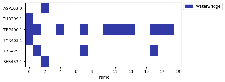
We can also analyze the water bridge interactions using a barcode plot.
fp.plot_barcode(figsize=(8, 3))
<Axes: xlabel='Frame'>
We can also visualize water-mediated interactions using the LigNetwork plot.
Here we can also see the water bridges with higher orders, where the water molecules interact
with each other thus building water bridges.
Tip
The threshold for interactions to be displayed in fp.plot_lignetwork() is 0.3. Thus only interactions with an occurence of more than 30 % will appear with the default settings, so don’t forget to adjust the threshold if you want to see interactions with lower occurence.
ligand_mol = plf.Molecule.from_mda(ligand_selection)
view = fp.plot_lignetwork(ligand_mol, threshold=0.05)
view
We can also visualize water-mediated interactions in 3D with the plot_3d function. Here is an example of the water-mediated interaction between the protein and ligand present in frame/pose 0.
Note
For plot_3d we need to provide the protein, ligand and water objects as plf.Molecule,
thus if you’re using an MD trajectory, a conversion from the mda.AtomGroup selection
which we used for fp.run() may be required:
# preparation for MD trajectories only
frame = 2
u.trajectory[frame]  # seek frame to update coordinates of atomgroup objects
ligand_mol = plf.Molecule.from_mda(ligand_selection, use_segid=fp.use_segid)
protein_mol = plf.Molecule.from_mda(protein_selection, use_segid=fp.use_segid)
water_mol = plf.Molecule.from_mda(water_selection, use_segid=fp.use_segid)
frame = 2
view = fp.plot_3d(ligand_mol, protein_mol, water_mol, frame=frame)
view
3Dmol.js failed to load for some reason. Please check your browser console for error messages.
<prolif.plotting.complex3d.Complex3D at 0x789cc29874d0>
You can also compare different poses/frames, please refer to the relevant Tutorials and
simply add water_mol in the plot_3d call.
Water Bridge Interaction Metadata#
The current example showed if specific water bridge interactions are present or not during the simulation. During the analysis, some metadata about the interaction is stored:
the indices of atoms involved in each component (ligan, protein or water),
the “order” of the water-mediated interaction, i.e. how many water molecules are involved in the bridge,
the residue identifier of the water molecules,
the role of the ligand and protein (H-bond acceptor or donor),
distances for each HBond interaction forming the bridge (and their sum).
frame = 0
all_interaction_data = fp.ifp[frame].interactions()
next(all_interaction_data)
InteractionData(ligand=ResidueId(QNB, 1, 2), protein=ResidueId(TRP, 400, 1), interaction='WaterBridge', metadata={'indices': {'ligand': (15,), 'protein': (23,), 'TIP383.3': (0, 1, 2)}, 'parent_indices': {'ligand': (15,), 'protein': (1362,), 'water': (56, 54, 55)}, 'water_residues': (ResidueId(TIP3, 83, 3),), 'order': 1, 'ligand_role': 'HBAcceptor', 'protein_role': 'HBAcceptor', 'distance_ligand_TIP383.3': 2.67114215102955, 'DHA_angle_ligand_TIP383.3': 162.19388273134385, 'distance_TIP383.3_protein': 2.723435581996723, 'DHA_angle_TIP383.3_protein': 174.91691520733102, 'distance': 5.3945777330262725})
Next we show how to access and process the metadata stored after the calculation of the interactions, using a pandas Dataframe for convenience.
all_metadata = []

for frame, ifp in fp.ifp.items():
    for interaction_data in ifp.interactions():
        if interaction_data.interaction == "WaterBridge":
            flat = {
                "frame": frame,
                "ligand_residue": interaction_data.ligand,
                "protein_residue": interaction_data.protein,
                "water_residues": " ".join(
                    map(str, interaction_data.metadata["water_residues"])
                ),
                "order": interaction_data.metadata["order"],
                "ligand_role": interaction_data.metadata["ligand_role"],
                "protein_role": interaction_data.metadata["protein_role"],
                "total_distance": interaction_data.metadata["distance"],
            }
            all_metadata.append(flat)

df_metadata = pd.DataFrame(all_metadata)
df_metadata
| frame | ligand_residue | protein_residue | water_residues | order | ligand_role | protein_role | total_distance | |
|---|---|---|---|---|---|---|---|---|
| 0 | 0 | QNB1.2 | TRP400.1 | TIP383.3 | 1 | HBAcceptor | HBAcceptor | 5.394578 |
| 1 | 0 | QNB1.2 | THR399.1 | TIP383.3 TIP317.3 | 2 | HBAcceptor | HBAcceptor | 8.450708 |
| 2 | 0 | QNB1.2 | TYR403.1 | TIP383.3 TIP317.3 | 2 | HBAcceptor | HBDonor | 8.791619 |
| 3 | 1 | QNB1.2 | TRP400.1 | TIP383.3 | 1 | HBAcceptor | HBAcceptor | 6.063980 |
| 4 | 1 | QNB1.2 | CYS429.1 | TIP383.3 | 1 | HBAcceptor | HBDonor | 6.379684 |
| 5 | 2 | QNB1.2 | ASP103.0 | TIP390.3 | 1 | HBDonor | HBAcceptor | 5.978124 |
| 6 | 2 | QNB1.2 | SER433.1 | TIP390.3 TIP393.3 TIP357.3 | 3 | HBDonor | HBAcceptor | 11.927196 |
| 7 | 4 | QNB1.2 | TRP400.1 | TIP383.3 | 1 | HBAcceptor | HBAcceptor | 6.092165 |
| 8 | 7 | QNB1.2 | TRP400.1 | TIP383.3 | 1 | HBAcceptor | HBAcceptor | 5.477529 |
| 9 | 7 | QNB1.2 | CYS429.1 | TIP383.3 | 1 | HBAcceptor | HBDonor | 6.179404 |
| 10 | 10 | QNB1.2 | TRP400.1 | TIP383.3 | 1 | HBAcceptor | HBAcceptor | 5.277520 |
| 11 | 11 | QNB1.2 | TRP400.1 | TIP383.3 | 1 | HBAcceptor | HBAcceptor | 6.317302 |
| 12 | 12 | QNB1.2 | TRP400.1 | TIP383.3 | 1 | HBAcceptor | HBAcceptor | 5.743704 |
| 13 | 13 | QNB1.2 | TRP400.1 | TIP383.3 | 1 | HBAcceptor | HBAcceptor | 5.826089 |
| 14 | 16 | QNB1.2 | TRP400.1 | TIP386.3 | 1 | HBAcceptor | HBAcceptor | 5.682423 |
| 15 | 16 | QNB1.2 | CYS429.1 | TIP386.3 | 1 | HBAcceptor | HBDonor | 6.286966 |
| 16 | 17 | QNB1.2 | TRP400.1 | TIP386.3 | 1 | HBAcceptor | HBAcceptor | 5.769556 |
| 17 | 18 | QNB1.2 | TRP400.1 | TIP3680.10 | 1 | HBAcceptor | HBAcceptor | 6.032010 |
We can now use this information to access interactions of orders 2 and 3 only to perform further analysis.
# count the occurence of each water residue in bridged interactions of higher order
(
    df_metadata[df_metadata["order"].isin([2, 3])]["water_residues"]
    .str.split(" ")
    .explode()
    .value_counts()
)
water_residues
TIP383.3    2
TIP317.3    2
TIP390.3    1
TIP393.3    1
TIP357.3    1
Name: count, dtype: int64